2D real time visualization: waveforms
Live video coding: animating a waveform
Click on this button to mute or unmute this video or press UP or DOWN buttons to increase or decrease volume level.
Downloads and transcripts
Video
Download video fileTranscripts
Do try on and study the code in the JSBin example created during the Live Coding Video
2D real time visualizations: waveforms
Introduction
WebAudio offers an Analyser node that provides real-time frequency and time-domain analysis information. It leaves the audio stream unchanged from the input to the output, but allows us to acquire data about the sound signal being played. This data is easy for us to process since complex computations such as Fast Fourier Transforms are being executed, behind the scenes,.
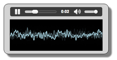
Example 1: audio player with waveform visualization
Do things in order – Select the audio context AND the canvas context, build the audio graph, and run the animation loop
Typical operations to perform once the HTML page is loaded:
- window.onload = function() {
- // get the audio context
- audioContext= …;
- // get the canvas, its graphic context…
- canvas = document.querySelector(“#myCanvas”);
- width = canvas.width;
- height = canvas.height;
- canvasContext = canvas.getContext(‘2d’);
- // Build the audio graph with an analyser node at the end
- buildAudioGraph();
- // starts the animation at 60 frames/s
- requestAnimationFrame(visualize);
- };
Step 1 – build the audio graph with an analyser node at the end
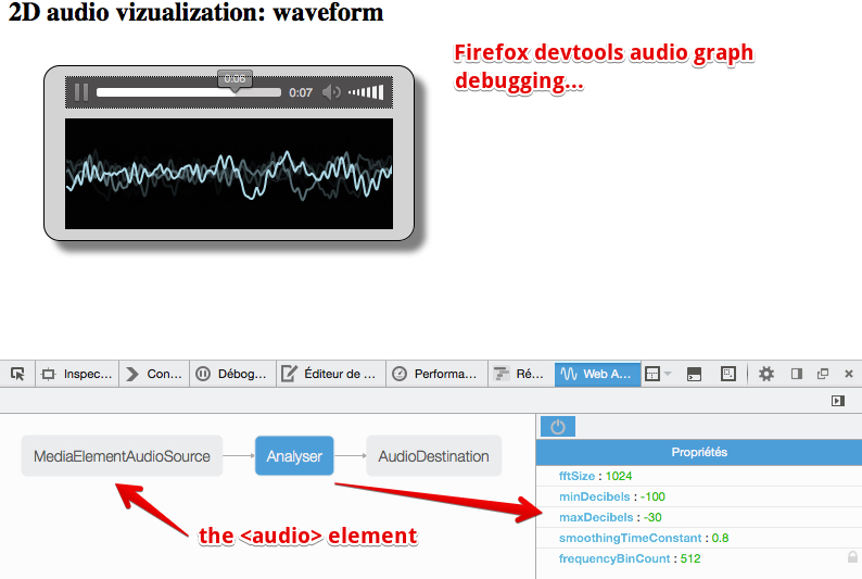
If we want to visualize the sound that is coming out of the speakers, we have to put an analyser node at almost the end of the sound graph. Example 1 shows a typical use: an <audio> element, a MediaElementElementSource node connected to an Analyser node, and the analyser node connected to the speakers (audioContext.destination). The visualization is a graphic animation that uses the requestAnimationFrame API presented in HTML5 part 1, Week 4.
Typical code for building the audio graph:
HTML code:
- <audio src=“http://mainline.i3s.unice.fr/mooc/guitarRiff1.mp3”
- id=“player” controls loop crossorigin=“anonymous”>
- </audio>
- <canvas id=“myCanvas” width=300 height=100></canvas>
JavaScript code:
- function buildAudioGraph() {
- var mediaElement = document.getElementById(‘player’);
- var sourceNode = audioContext.createMediaElementSource(mediaElement);
- // Create an analyser node
- analyser = audioContext.createAnalyser();
- // set visualizer options, for lower precision change 1024 to 512,
- // 256, 128, 64 etc. bufferLength will be equal to fftSize/2
- analyser.fftSize = 1024;
- bufferLength = analyser.frequencyBinCount;
- dataArray = new Uint8Array(bufferLength);
- sourceNode.connect(analyser);
- analyser.connect(audioContext.destination);
- }
With the exception of lines 8-12, where we set the analyser options (explained later), we build the following graph:
Step 2 – write the animation loop
The visualization itself depends on the options which we set for the analyser node. In this case we set the FFT size to 1024 (FFT is a kind of accuracy setting: the bigger the value, the more accurate the analysis will be. 1024 is common for visualizing waveforms, while lower values are preferred for visualizing frequencies). Here is what we set in this example:
- analyser.fftSize = 1024;
- bufferLength = analyser.frequencyBinCount;
- dataArray = new Uint8Array(bufferLength);
- Line 2: we set the size of the FFT,
- Line 3: this is the byte array that will contain the data we want to visualize. Its length is equal to fftSize/2.
When we build the graph, these parameters are set – effectively as constants, to control the analysis during play-back .
Here is the code that is run 60 times per second to draw the waveform:
- function visualize() {
- // 1 – clear the canvas
- // like this: canvasContext.clearRect(0, 0, width, height);
- // Or use rgba fill to give a slight blur effect
- canvasContext.fillStyle = ‘rgba(0, 0, 0, 0.5)’;
- canvasContext.fillRect(0, 0, width, height);
- // 2 – Get the analyser data – for waveforms we need time domain data
- analyser.getByteTimeDomainData(dataArray);
- // 3 – draws the waveform
- canvasContext.lineWidth = 2;
- canvasContext.strokeStyle = ‘lightBlue’;
- // the waveform is in one single path, first let’s
- // clear any previous path that could be in the buffer
- canvasContext.beginPath();
- var sliceWidth = width / bufferLength;
- var x = 0;
- for(var i = 0; i < bufferLength; i++) {
- // dataArray values are between 0 and 255,
- // normalize v, now between 0 and 1
- var v = dataArray[i] / 255;
- // y will be in [0, canvas height], in pixels
- var y = v * height;
- if(i === 0) {
- canvasContext.moveTo(x, y);
- } else {
- canvasContext.lineTo(x, y);
- }
- x += sliceWidth;
- }
- canvasContext.lineTo(canvas.width, canvas.height/2);
- // draw the path at once
- canvasContext.stroke();
- // once again call the visualize function at 60 frames/s
- requestAnimationFrame(visualize);
- }
Explanations:
- Lines 9-10: we ask for the time domain analysis data. The call to getByteTimeDomainData(dataArray) will fill the array with values corresponding to the waveform to draw. The returned values are between 0 and 255. See the specification for details about what they represent exactly in terms of audio processing.
Below are other examples that draw waveforms.
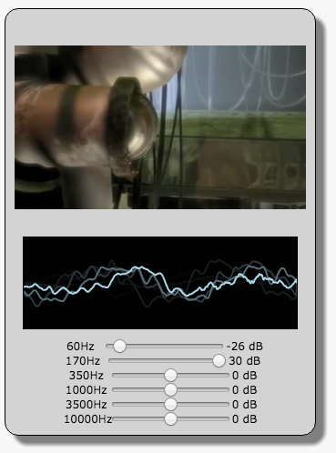
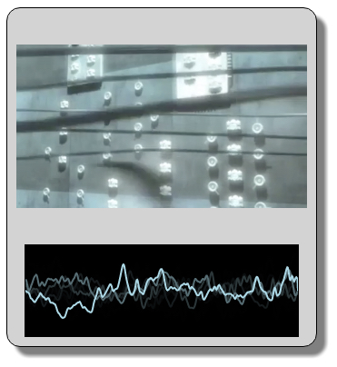
Example 2: video player with waveform visualization
Using a <video> element is very similar to using an <audio> element. We have made no changes to the JavaScript code here; we Just changed “audio” to “video” in the HTML code.
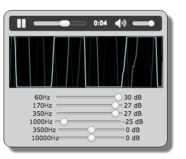
Example 3: both examples, this time with the graphic equalizer
Adding the graphic equalizer to the graph changes nothing, we visualize the sound that goes to the speakers. Try lowering the slider values – you should see the waveform changing.