2D real time visualization: frequencies
First typical example
This time, instead of a waveform we want to visualize an animated bar chart. Each bar will correspond to a frequency range and ‘dance’ in concert with the music being played.
- The frequency range depends upon the sample rate of the signal (the audio source) and on the FFT size. While the sound is being played, the values change and the bar chart is animated.
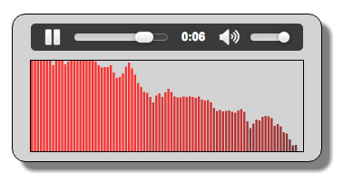
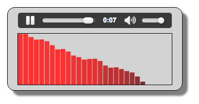
- The number of bars is equal to the FFT size / 2 (left screenshot with size = 512, right screenshot with size = 64).
- In the example above, the Nth bar (from left to right) corresponds to the frequency range N * (samplerate/fftSize). If we have a sample rate equal to 44100 Hz and a FFT size equal to 512, then the first bar represents frequencies between 0 and 44100/512 = 86.12Hz. etc. As the amount of data returned by the analyser node is half the fft size, we will only be able to plot the frequency-range to half the sample rate. You will see that this is generally enough as frequencies in the second half of the sample rate are not relevant.
- The height of each bar shows the strength of that specific frequency bucket. It’s just a representation of how much of each frequency is present in the signal (i.e. how “loud” the frequency is).
You do not have to master the signal processing ‘plumbing’ summarised above – just plot the reported values!
Enough said! Let’s study some extracts from the source code.
This code is very similar to Example 1 at the top of this page. We’ve set the FFT size to a lower value, and rewritten the animation loop to plot frequency bars instead of a waveform:
- function buildAudioGraph() {
- …
- // Create an analyser node
- analyser = audioContext.createAnalyser();
- // Try changing to lower values: 512, 256, 128, 64…
- // Lower values are good for frequency visualizations,
- // try 128, 64 etc.?
- analyser.fftSize = 256;
- …
- }
This time, when building the audio graph, we have used a smaller FFT size. Values between 64 and 512 are very common here. Try them in the JSBin example! Apart from the lines in bold, this function is exactly the same as in Example 1.
The new visualization code:
- function visualize() {
- // clear the canvas
- canvasContext.clearRect(0, 0, width, height);
- // Get the analyser data
- analyser.getByteFrequencyData(dataArray);
- var barWidth = width / bufferLength;
- var barHeight;
- var x = 0;
- // values go from 0 to 255 and the canvas heigt is 100. Let’s rescale
- // before drawing. This is the scale factor
- heightScale = height/128;
- for(var i = 0; i < bufferLength; i++) {
- // between 0 and 255
- barHeight = dataArray[i];
- // The color is red but lighter or darker depending on the value
- canvasContext.fillStyle = ‘rgb(‘ + (barHeight+100) + ‘,50,50)’;
- // scale from [0, 255] to the canvas height [0, height] pixels
- barHeight *= heightScale;
- // draw the bar
- canvasContext.fillRect(x, height–barHeight/2, barWidth, barHeight/2);
- // 1 is the number of pixels between bars – you can change it
- x += barWidth + 1;
- }
- // once again call the visualize function at 60 frames/s
- requestAnimationFrame(visualize);
- }
Explanations:
- Line 6: this is different to code which draws a waveform! We ask for byteFrequencyData (vs byteTimeDomainData earlier) and it returns an array of fftSize/2 values between 0 and 255.
- Lines 16-29: we iterate on the value. The x position of each bar is incremented at each iteration (line 28) adding a small interval of 1 pixel between bars (you can try different values here). The width of each bar is computed at line 8.
- Line 14: we compute a scale factor to be able to display the values (ranging from 0 to 255) in direct proportion to the height of the canvas. This scale factor is used in line 23, when we compute the height of the bars we are going to draw.
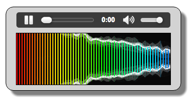
Another example: achieving more impressive frequency visualization
Example at JSBin with a different look for the visualization: The example is given as is, read the source code and try to understand how the drawing of the frequency is done.
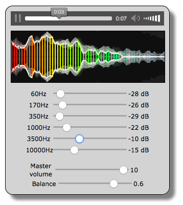
And here is the audio graph for this example:
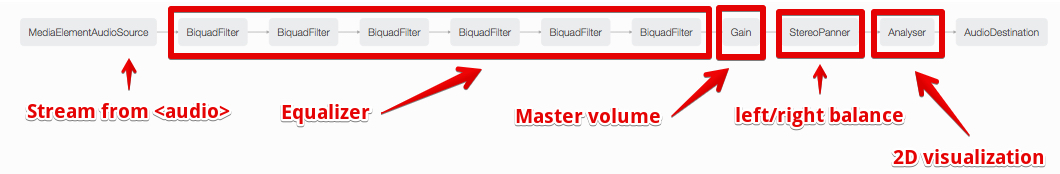
Source code from this example’s the buildAudioGraph function:
- function buildAudioGraph() {
- var mediaElement = document.getElementById(‘player’);
- var sourceNode = audioContext.createMediaElementSource(mediaElement);
- // Create an analyser node
- analyser = audioContext.createAnalyser();
- // Try changing for lower values: 512, 256, 128, 64…
- analyser.fftSize = 1024;
- bufferLength = analyser.frequencyBinCount;
- dataArray = new Uint8Array(bufferLength);
- // Create the equalizer, which comprises a set of biquad filters
- // Set filters
- [60, 170, 350, 1000, 3500, 10000].forEach(function(freq, i) {
- var eq = audioContext.createBiquadFilter();
- eq.frequency.value = freq;
- eq.type = “peaking”;
- eq.gain.value = 0;
- filters.push(eq);
- });
- // Connect filters in sequence
- sourceNode.connect(filters[0]);
- for(var i = 0; i < filters.length – 1; i++) {
- filters[i].connect(filters[i+1]);
- }
- // Master volume is a gain node
- masterGain = audioContext.createGain();
- masterGain.value = 1;
- // Connect the last filter to the speakers
- filters[filters.length – 1].connect(masterGain);
- // for stereo balancing, split the signal
- stereoPanner = audioContext.createStereoPanner();
- // connect master volume output to the stereo panner
- masterGain.connect(stereoPanner);
- // Connect the stereo panner to analyser and analyser to destination
- stereoPanner.connect(analyser);
- analyser.connect(audioContext.destination);
- }
